Exercise: Atomistic Simulation of Biomolecular function, Part 1
Leonard Heinz
Tutorial adapted from Bert de Groot.
Contents
Introduction
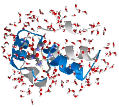
In this part of the exercise, we will set up a simulation of a biological
macromolecule: a small protein.
Proteins are nature's universal machines. For example, they are used as building blocks (e.g. collagen in skin, bones and teeth), transporters (e.g. hemoglobin as oxygen transporter in the blood), as reaction catalysts (enzymes like lysozyme that catalyse the breakdown of
sugars), and as nano-machines (like myosin that is at the basis of muscle contraction). The protein's structure or molecular architecture is sufficient
for some of these functions (like for example in the case of collagen), but for most others the function is intimately linked to internal dynamics. In these
cases, evolution has optimised and fine-tuned the protein to exhibit exactly that type of dynamics that is essential for its function. Therefore, if we want
to understand protein function, we often first need to understand its
dynamics (see references below).
Unfortunately, there are no experimental techniques available to study protein dynamics at the atomic resolution at the physiologically
relevant time resolution (that can range from seconds or milliseconds down to nanoseconds or even picoseconds). Therefore, computer simulations are
employed to numerically simulate protein dynamics.
We will use the GROMACS simulation package for this.
Today, we will simulate the dynamics of a small, typical protein domain: the B1 domain of protein G. B1 is one of the domains
of protein G, a member of an important class of proteins, which form IgG binding receptors on the surface of certain Staphylococcal and
Streptococcal strains. These proteins allow the pathogenic bacterium to evade the host immune response by coating the invading bacteria
with host antibodies, thereby contributing significantly to the pathogenicity
of these bacteria.
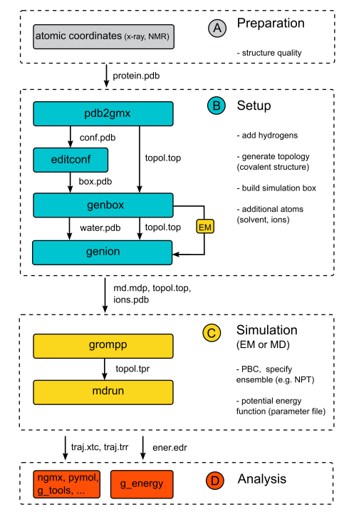
We will now follow a standard protocol to run a typical MD simulation of a
protein in a box of water in gromacs. The individual steps are summarized in a flowchart on the right site.
Go back to Contents
Preparation (A)
Before a simulation can be started, an initial structure of the protein is required. Fortunately, the structure of the B1 domain of
protein G has been solved experimentally, both by x-ray crystallography and NMR. Experimentally solved protein structures are
collected and distributed by the Protein Data Bank (PDB). Please open
this link in a new browser
window. To download
the structure select "PDB File" under "Download Files". When prompted, select "save to disk", and save the file
to save it in a new folder, e.g, gromacs_tutorial_p1 (click here if that does not work). To have a look at the contents of the file, on the unix prompt, type:
The file starts with general information about the protein, about the
structure, and about the experimental techniques used to determine the
structure, as well as literature references where the structure is described
in detail. (in "more", press the spacebar to scroll). The data file contains the atomic coordinates of our protein structure with one line per atom. (quit the "more" program by pressing "q").
Now we can have a look at the structure:
to visualise the structure.
We now see a so-called wireframe
representation of the protein structure: atoms (with different colors
for the different chemical elements: cyan for carbon; red for oxygen
and blue for nitrogen) are not shown directly, but the
bonds between atoms are shown as lines. Under Graphics -> Representations -> Drawing Method, also try
other representations such as "Licorice", "VDW" and "New Cartoon". Exit rasmol under File -> Quit.
Question: Why do we start our MD
simulations from the experimentally determined 3D structure? Isn't it enough to know the protein's amino acid sequence?
Go back to Contents
Setup (B)
We will now prepare the protein structure to be simulated in gromacs. Although we now have a starting structure for our protein, one might
have noticed that hydrogen atoms (which would appear white) are still missing from the
structure. This is because hydrogen atoms contain too few electrons to
be observed by x-ray crystallography at moderate resolutions. Also,
gromacs requires a molecular description (or topology) of the
molecules to be simulated before we can start, containing information
on e.g. which atoms are covalently bonded and other physical information. Both the generation of
hydrogen atoms and writing of the topology can be done with the
gromacs program pdb2gmx:
gromacs_2018
gmx pdb2gmx -f 1PGB.pdb -o conf.pdb
when prompted for the force-field to be used, choose the number corresponding
to the OPLS-AA/L all-atom force field, and SPC/E for water. View the result with:
See the added hydrogens? The topology file written by pdb2gmx is called "topol.top". Have a
look at the contents of the file using:
you will see a list of all the atoms (with masses, charges), followed
by bonds (covalent bonds connecting the atoms), angles, dihedral
angles etc. Near the very end of the topology (in the "[molecules]"
section) there is a summary of the simulation system, including the
protein and 24 crystallographic water molecules.
The topology file thus contains all the physical information about all
interactions between the atoms of the protein (bonds, angles, torsion
angles, Lennard-Jones interactions and electrostatic interactions).
The next step in setting up the simulation system is to solvate the
protein in a water box, to mimick a physiological environment. For that, we first need to define a
simulation box. In this case we will generate a rectangular box with
the box-edges at least 7 Angstroms apart from the protein surface:
gmx editconf -f conf.pdb -o box.pdb -d 0.7
(note that gromacs uses units of nanometers). View the result
with
and, in the VMD terminal, type:
Now, exit VMD and fill the simulation box with SPC water using gmx solvate:
gmx solvate -cp box.pdb -cs spc216 -o water.pdb -p topol.top
Again, view the output (water.pdb) with VMD. Now the simulation
system is almost ready. Before we can start the dynamics, we must
perform an energy minimisation.
Question: Why do we need an energy
minimisation step? Wouldn't the crystal structure as it is be a good starting
point for MD as it is?
For the energy minimisation, we need a parameter file,
specifying which type of minimisation should be carried out, the
number of steps, etc. For your convenience a file called "em.mdp" has
already been prepared and can be downloaded from here. View the file
with "more" to see its contents. We use the gromacs preprocessor to
prepare our energy minimisation:
gmx grompp -f em.mdp -c water.pdb -p topol.top -o em.tpr -maxwarn 2
This collects all the information from em.mdp, the coordinates from
water.pdb and the topology from topol.top, checks if the contents are
consistent and writes a unified output file: em.tpr, which will be
used to carry out the minimisation:
gmx mdrun -v -s em.tpr -c em.pdb
The output shows that already the initial energy was rather low, so
in this case there were hardly any bad contacts. Having a look at
"em.pdb" shows that the structure hardly changed during
minimisation.
The careful user may have noticed that grompp gave a warning:
System has non-zero total charge: -4.
Before we continue with the dynamics, we should neutralise
this net charge of the simulation system. This
is to prevent artefacts that would arise as a side effect caused by
the periodic boundary conditions used in the simulation. A net charge
would result in an electrostatic repulsion between neighbouring
periodic images. Therefore, 4 sodium ions will be added to the system:
gmx genion -s em.tpr -o ions.pdb -np 4 -p topol.top
Select the water group ("SOL"), and 4 water molecules
will be replaced by sodium ions.
The output (ions.pdb) can be checked with VMD. To better see the
ions in VMD, select Graphics -> Representations, type "protein" in the "Select Atoms" field and confirm by pressing enter; then create a new representation, select the ions with "name NA", press enter and choose "VDW" as the drawing method.
Go back to Contents
Simulation (C)
Just to be on the safe side, we repeat the energy minimisation, now with the ions included
(remember to (re)run grompp to create a new run input file whenever
changes to the topology, or coordinates have been made):
gmx grompp -f em.mdp -c ions.pdb -p topol.top -o em.tpr -maxwarn 2
gmx mdrun -v -s em.tpr -c em.pdb
Now we have all that is required to start the dynamics. Again, a
parameter file has been prepared for the simulation, and can be
downloaded here. Please browse
through the file "md.mdp" (using "more") to get an idea of the
simulation parameters. The gromacs online manual describes all
parameters in detail here.
Please don't worry in this stage about all individual parameters,
we've chosen common values typical for protein simulations.
Again, we use the gromacs preprocessor to prepare the simulation:
gmx grompp -f md.mdp -c em.pdb -p topol.top -o md.tpr -maxwarn 2
and start the simulation!
gmx mdrun -v -s md.tpr -c md.pdb -nice 0
The simulation is running now, and depending on the speed and load of
the computer, the simulation will run for a number of minutes.
Question: How do the parts of energy
minimization and MD simulation differ (with reference to energy landscapes)?
Go back to Contents
Analysis of a gromacs simulation (D)
If the simulation has finished, we can start analysing
the results. Let us first see which kind of files have been written by
the simulation (mdrun):
We see the following files:
- traj_comp.xtc - the trajectory to be used for analyses
- traj.trr - the trajectory to be used for a restart in case of a crash
- ener.edr - energies
- md.log - a LOG file of mdrun
- md.pdb - the final coordinates of the simulation
The first analysis step during or after a simulation is usually a
visual inspection of the trajectory. For this we will use VMD.
Select a group of your interest using the "Representations"-menue. You can, e.g., use the keywords "protein", "water", "name NA" and the logical operators "and", "or", "not". Click the play-button in the main window to see the trajectory. We can see that the protein and its surroundings undergo thermal
fluctuations, but overall, the protein structure is rather stable, as
would be expected on such timescales.
For a more quantitative analysis
on the protein fluctuations, we can view how fast and how far the
protein deviates from the starting (experimental) structure:
gmx rms -s md.tpr -f traj_comp.xtc
When prompted for groups to be analysed, type "1 1". gmx rms has
written a file called "rmsd.xvg", which can be viewed with:
We see the Root Mean Square Deviation (rmsd) from the starting
structure, averaged over all protein atoms, as a function of time.
Question: Why is there an intial rise in the rmsd?
The simulation not only yields information on the structural
properties of the simulation, but also on the energetics. With the
program gmx energy the energies written by mdrun can be analysed:
Select "Potential" and end your selection by pressing enter twice, View the result with:
As can be seen, the total potential energy initially rises rapidly after
which it relaxes again.
Question: Can you think of an explanation for
this behaviour?
Please repeat the energy analysis for a number of different energy
terms to obtain an impression of their behaviour.
Question: Do you think the length of our
simulation is sufficient to provide a faithful picture of the protein's
conformations at equillibrium?
You've probably noticed that in the simulation about only ten percent of the
system that was simulated consisted of protein, the rest was water. As we are
mainly interested in the protein's motions and not so much in the surrounding
water, one could ask if we couldn't forget about the water and rather simulate
the protein. That way, we could reach ten times longer simulations with the
same computational effort!
Question: Why do you think that it is
important to include explicit solvent in the simulation of a protein?
Continue with part 2.
Optional exercises
To check if your assumption is correct, repeat the simulation of protein G,
this time without solvent (to observe the effect more clearly, increase the
length of the simulation by changing "nsteps" in the file "md.mdp" by e.g. a
factor of ten).
Question: What are the main differences to the
protein's structure and dynamics as compared to the solvent simulation?
(Hint: use programs like gmx rms and gmx gyrate to analyse both simulations).
Go back to Contents
Further references:
Principles of protein structure and basic in biophysics and biochemistry:
- Stryer, Biochemistry
- Voet, Fundamentals of Biochemistry Rev. Ed.
- Cantor and Schimmel, Biophysical Chemistry Part I: The conformation of biological macromolecules
Computer simulations and molecular dynamics:
- M. Karplus and A. McCammon. Molecular Dynamics simulations of
biomolecules Nature structural biology 9: 646-652 (2002).[link]
- D.C. Rapaport. The Art of Molecular Dynamics Simulations - 2nd edn
Cambridge University Press (2004).
Advanced reading:
- H. Scheraga, M. Khalili and A. Liwo. Protein-Folding Dynamics:
Overview of Molecular Simulation Techniques Annual Review of Physical Chemistry 58: 57-83 (2007).[link]
- K Henzler-Wildman and D Kern. Dynamic personalities of proteins Nature 450: 964-972 (2007).
- K A Sharp and B Honig. Electrostatic Interactions in Macromolecules: Theory and Applications, Annual Review of Biophysics and Biophysical Chemistry 19: 301-332 (1990).
- F M Richards. Areas, Volumes, Packing, and Protein Structure Annual Review of Biophysics and Bioengineering 6: 151-176 (1977).
- K A Dill, S B Ozkan, M Scott Shell and T R Weikl. The Protein Folding Problem Annual Review of Biophysics 37: 289-316 (2008).
For questions or feedback please contact Helmut Grubmüller / hgrubmu@gwdg.de or Leonard Heinz / lheinz@gwdg.de