Exercise: Atomistic Simulation of Biomolecular function, Part 2

To start the simulations, ssh to the daint-cluster:

ela
ssh daint

Once done, load the daint hybrid modules and gromacs, the simulation program that we are going to use today.

module load daint-gpu
module load GROMACS

To make copying the simulation results to your local machine easier, create a new folder in which all simulations will be carried out.

mkdir gromacs_tutorial
cd gromacs_tutorial

The simulation input-files have already been prepared for you. You can download them using this little script. Download the script, e.g. using wget

wget http://www2.mpibpc.mpg.de/groups/grubmueller/Lugano_Tutorial/part2/download_files.bash

Then make the script executable and use it to download the other files.

chmod +x download_files.bash
bash download_files.bash

You will find that a few files were downloaded and two directories, "pull1" and "pull2", were created. Each folder contains a set of MD parameters (.mdp-file) and a jobscript that we are going to use later to run the simulation on the cluster. Before we can do that, we need to run the gromacs-preprocessor for each simulation.

cd pull1
gmx grompp -f pull1.mdp -c ../start.gro -p ../topol.top -n ../index.ndx -o pull1.tpr

Change the names to "pull2" in the last line and also run the preprocessor (gmx grompp) in "pull2".

Now we are ready to submit the simulations to daint. Use, e.g.,

sbatch jobscript1.bash

to submit the first simulation in "pull1". Do the same in the folder "pull2" respectively.

You can use the command

squeue -u classXX

(substitute classXX by the username connected to your machine, look at the start of every line in the terminal) to check if your jobs are already running. If so, check the output-files in the folders ("pull1" and "pull2") for any errors. If your jobs are still queued, keep the terminal open and periodically check their status while working on part 1, so that errors can be caught early. If errors occur, don't hesitate to ask the tutor.

Start with part 1 of the tutorial, which you can entirely perform on the local machine (so use a new terminal).

Understanding the simulation setup

cp -r /scratch/snx3000/classXX/gromacs_tutorial ~/.

Then open a new terminal on your local machine and copy the files

scp -r classXX@ela.cscs.ch:~/gromacs_tutorial ~/.

Finally, you should delete gromacs_tutorial from the home-directory of the cluster.

Should the simulations have failed for any reason, you can try to fix the problem and run again or, if there is a lack of time, download prepared simulation results of pull1 and pull2.

All the remaining steps are ment to be performed in your local copy of gromacs_tutorial. You can logout from the cluster.

Question: With your knowledge from part 1 of the tutorial, can you figure out what the files "start.gro", "topol.top", "index.ndx", as well as the .mdp-files are good for?

Question: Look at "pull1.mdp" and "pull2.mdp". At which parameters do the two simulations differ? The pulling-options are set at the bottom of each file. Use the gromacs manual to find out where the pulling forces were applied in the simulations, which spring constants and which pulling speeds were used.

Analyzing the simulation results

Inspect both simulated trajectories visually using VMD, e.g. with

vmd start.gro pull1/pull1.xtc

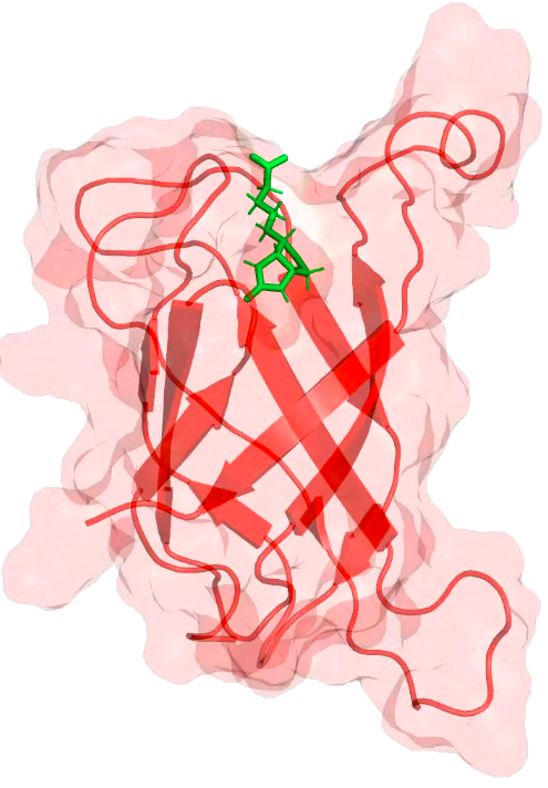
The selection-keywords "protein" and "resname BTN" will be useful; also change the drawing methods to something appropriate, e.g., "New Cartoon" for the protein and "Licorice" for biotin.

Question: Do you see the unbinding of biotin from streptavidin? Can you spot intermediate binding states in the trajectory with the slower pulling?

For both simulations, the pulling forces were recorded in "pull1/pull1_pullf.xvg" and "pull2/pull2_pullf.xvg", respectively. Plot both of them versus the simulated time, e.g., with

xmgrace pull1/pull1_pullf.xvg

and determine the rupture forces.

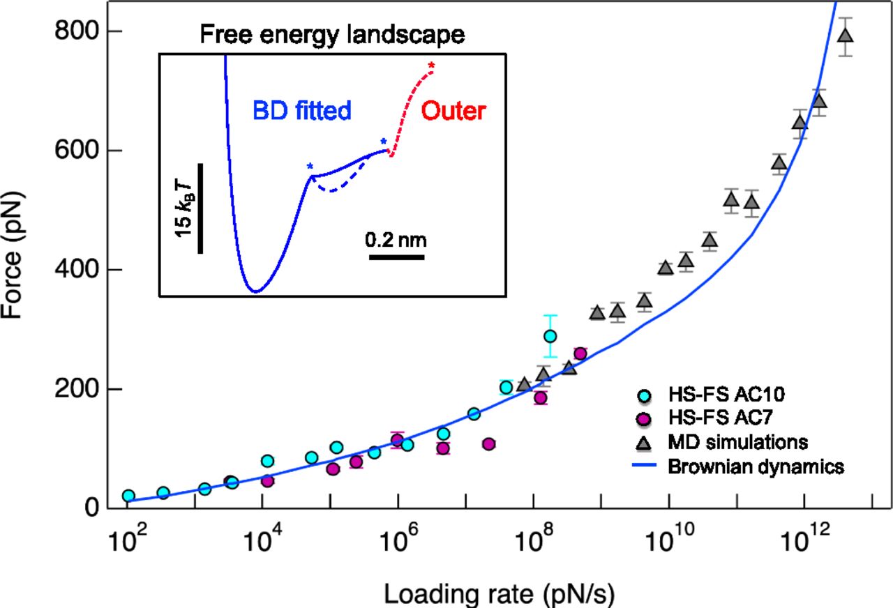
On the right you see a plot of the rupture forces depending on the loading rate from experiments, brownian dynamics and MD simulations from Rico et al. [Proc. Nat. Acad. Sci., 2019]. Calculate the loading rate (product of the spring constant and the pulling velocity) for each of your simulations and compare your results to the figure. Hint: Gromacs standard units are nm for distances, ps for times and kJ/mol for energies.

Question: How do your results compare to those in the figure? What could be possible reasons for deviations?

Question: Why is it so difficult to achieve overlap between simulation results and experiments for pulling?

Further references and advanced reading

• Rico F, Russek A, Gonzalez L, Grubmüller H, Scheuring S. Heterogeneous and rate-dependent streptavidin-biotin unbinding revealed by high-speed force spectroscopy and atomistic simulations. Proc. Nat. Acad. Sci. 116(4), 6594-6601 (2019) [link]